Kolmogorov’s “5/3” Law

This is a follow-up to my earlier post on “named” numbers; the text is mostly cannibalised from my book; I refer the reader to the book (available for free download) for bibliography, etc.

The famous mathematician Andrei Kolmogorov was the author of what remains the most striking and beautiful example of a dimensional analysis argument in mathematics. The deduction of his seminal “” law for the energy distribution in the turbulent fluid [A. N. Kolmogorov, Local structure of turbulence in an incompressible fluid for very large Reynolds numbers, Doklady Acad Sci. USSR 31 (1941) 301-305] is so simple that it can be done in a few lines.

I was lucky to study at a good secondary school where my physics teacher (Anatoly Mikhailovich Trubachov, to whom I express my eternal gratitude) derived the “” law in one of his improvised lectures. In my exposition, I borrow some details from Arnold and Ball (where I have also picked the idea of using a woodcut by Katsushika Hokusai as an illustration).

Multiple scales in the motion of a fluid, from a woodcut by Katsushika Hokusai, The Great Wave off Kanagawa (from the series Thirty-six View sof Mount Fuji, 1823–1829). This image is much beloved by chaos scientists. Source: Wikipedia Commons. Public domain.

The turbulent flow of a liquid consists of vortices; the flow in every vortex is made of smaller vortices, all the way down the scale to the point when the viscosity of the fluid turns the kinetic energy of motion into heat. If there is no influx of energy (like the wind whipping up a storm in Hokusai’s woodcut), the energy of the motion will eventually dissipate and the water will stand still.

So, assume that we have a balanced energy flow, the storm is already at full strength and stays that way. The motion of a liquid is made of waves of different lengths; Kolmogorov asked the question, what is the share of energy carried by waves of a particular length?

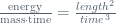
Here it is a somewhat simplified description of his analysis. We start by making a list of the quantities involved and their dimensions. First, we have the energy flow (let me recall, in our setup it is the same as the dissipation of energy). The dimension of energy is

(remember the formula for the kinetic energy of a moving material point?). It will be convenient to make all calculations per unit of mass. Then the energy flow has dimension

For counting waves, it is convenient to use the wave number, that is, the number of waves fitting into the unit of length. Therefore the wave number has dimension

Finally, the energy spectrum is the quantity such that, given the interval

between the two wave numbers, the energy (per unit of mass) carried by waves in this interval should be approximately equal to . Hence the dimension of is

To make the next crucial calculations, Kolmogorov made the major assumption that amounted to saying that

The way bigger vortices are made from smaller ones is the same throughout the range of wave numbers, from the biggest vortices (say, like a cyclone covering the whole continent) to a smaller one (like a whirl of dust on a street corner).

(This formulation is a bit cruder than most experts would accept; I borrow it from Arnold~\cite{chto).

Then we can assume that the energy spectrum , the energy flow and the wave number are linked by an equation which does not involve anything else. Since the three quantities involved have completely different dimensions, we can combine them only by means of an equation of the form

Here is a constant; since the equation should remain the same for small scale and for global scale events, the shape of the equation should not depend on the choice of units of measurements, hence should be dimensionless.

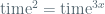
Let us now check how the equation looks in terms of dimensions:

After equating lengths with lengths and times with times, we have

which leads to a system of two simultaneous linear equations in and ,

This can be solved with ease and gives us

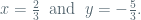
Therefore we come to Kolmogorov’s “” Law:

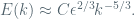
The dimensionless constant can be determined from experiments and happens to be pretty close to .

The status of this celebrated result is quite remarkable. In the words of an expert on turbulence, Alexander Chorin,

Nothing illustrates better the way in which turbulence is suspended between ignorance and light than the Kolmogorov theory of turbulence, which is both the cornerstone of what we know and a mystery that has not been fathomed.

The same spectrum […] appears in the sun, in the oceans, and in man­made machinery. The law is well verified experimentally and, by suggesting that not all scales must be computed anew in each problem, opens the door to practical modelling.

Arnold reminds us that the main premises of Kolmogorov’s argument remain unproven — after more than 60 years! Even worse, Chorin points to the rather disturbing fact that

Kolmogorov’s spectrum often appears in problems where his assumptions clearly fail. […] The law can now be derived in many ways, often under assumptions that are antithetical to Kolmogorov’s. Turbulence theory finds itself in the odd situation of having to build on its main result while still struggling to understand it.

Exercises for the reader

The history of dimensional analysis can be traced back at least to Froude’s Law of Steamship Comparisons used to great effect in D’Arcy Thompson’s book On Growth and Form for the analysis of speeds of animals:

The maximal speed of similarly designed steamships is proportional to the square root of their length.

William Froude (1810–1879) was the first to formulate reliable laws for the resistance that water offers to ships and for predicting their stability.

Exercise 1, moderate. Prove Froude’s Law.

Exercise 2, easy. Why does a mouse have (relatively) slimmer body build than an elephant?

Exercise 3, easy. Prove the following corollary of Froude’s Law:

The relative speed of a fish (that is, speed measured in numbers of its lengths covered by the fish per unit of time) is inverse proportional to the square root of its length.

This explains a well-known phenomenon: little fish in a stream appear to be very quick.

Exercise 4, even easier. Estimate, who is relatively faster: an ant or a racehorse?

A research project. Building on ideas from Exercise 2, develop a method for estimation of a maximal possible height of a tree of given species.

The problem is of serious practical value. To explain it to an Englishman, you have to mention just one word: Leylandii.

X Cupressocyparis leylandii : 35 meters and still growing.

For a foreigner, Wikipedia provides more detail:

The Leyland Cypress, X Cupressocyparis leylandii, is often referred to as just Leylandii. It is a fast-growing evergreen tree much used in horticulture, primarily for hedges and screens.

The Leyland Cypress is a hybrid between the Monterey Cypress, Cupressus macrocarpa, and the Nootka Cypress, Cupressus nootkatensis. The hybrid has arisen on nearly 20 separate occasions, always by open pollination. […]

Leyland Cypresses are commonly planted in gardens to provide a quick boundary or shelter hedge. However, their rapid growth (up to a metre per year), heavy shade and great potential height (often over 20 m tall in garden conditions, they can reach at least 35 m) make them a problem. In Britain they have been the source of a number of high profile disputes between neighbours, even leading to violence (and in one recent case, murder), because of their capacity to cut out light.

The problem is that no-one knows the maximal height of some of the latest hybrids — all known specimens continue to grow…